预训练框架|适配深度表型数据的 Transformer 基础模型 ukbFound:架构与源码解析
阅读提醒:好久不见👋,最近作者太忙了没怎么更新,现在来更新了🎉。本篇基于北京协和医学院的论文 A foundational model encodes deep phenotyping data and enables diverse downstream applications 以及其核心源码实现进行拆解。不同于常见的论文复述,本文试图回答:这篇论文的创新架构在代码层面是如何落地的?原文献中提到的强制掩码(Forced Masking)和分层掩码(Stratified Masking)是如何具体执行的?对于模型的可解释性和下游任务的鲁棒性,代码给出了怎样的答案?以及关于这种新的范式的论文套路如何去做的。(需要你有一定的对语言模型的背景理解以及对Transformer模型架构的了解,还有python编码等等知识) 笔者在阅读源码过程中发现了一些关键细节(如硬编码的疾病索引范围),这些细节在论文中并未完全展开,但对理解整个模型的数据流至关重要。如有兴趣探讨底层逻辑或获取相关代码分析脚本,欢迎邮箱联系📮笔者,全文约3w字。祝食用愉快~😳
导言:从 EHR 到 Deep Phenotyping 的范式转变
“ 近年来,精准医学的数据源正在从传统的电子病历(EHR)向 Deep Phenotyping(深度表型分析)演进。这个变化背后的核心矛盾很明确:传统的 EHR 数据虽然包含了诊断记录,但往往碎片化且缺乏早期的风险信号;而深度表型数据(如生物标志物、基因组、长期生活方式记录)虽然信息丰富,但其高维、异构且缺乏自然顺序的特点,使得传统的机器学习方法难以有效建模。 ”
解释一下:深度表型分析(Deep Phenotyping) 是通过整合多维数据对个体进行全面表征,包括:
- 生物标志物(血液指标、代谢物等)
- 生活方式(运动、睡眠、吸烟等)
- 饮食习惯(酒类、蔬果摄入等)
- 环境暴露
- 教育水平
图 1 去年的nature论文
在 npj Digital Medicine 上发表的这篇论文 “A foundational model encodes deep phenotyping data and enables diverse downstream applications” 中,作者提出了 ukbFound。它试图将医学表征学习从单一的“诊断代码预测”改造成一个能够理解复杂表型关联的语言级基础模型。
核心架构解析
论文试图解决什么问题?
ukbFound 的核心挑战在于如何将高度非结构化的医疗数据(如连续变量、多选问卷、缺失值)转化为 Transformer 能理解的形式,同时不引入错误的先验假设(如特征出现的先后顺序)。
图 2 ukbFound 架构总览
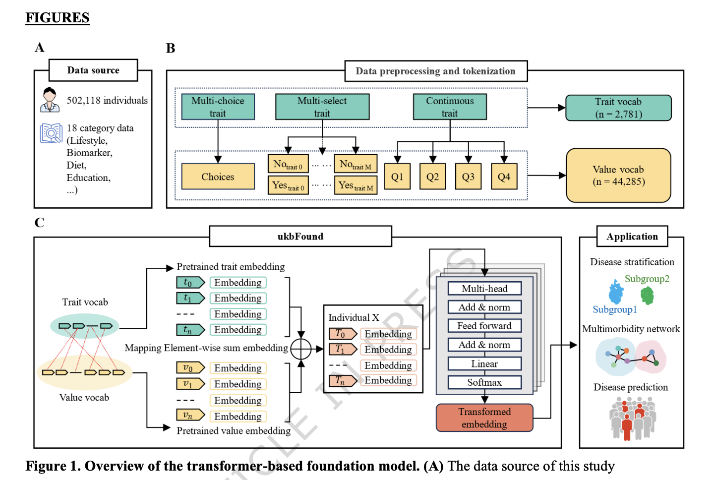
论文将特征处理划分为两个核心步骤:层次化 Tokenization 与 位置无关嵌入(Position-Free Embedding)。以及这篇论文对MLM训练方式进行了改进。下面将会详细说明:
第一部分:层次化 Tokenization
“原文: Hierarchical tokenization strategy. The heterogeneous data types underwent standardization through a dual-vocabulary tokenization framework comprising trait and value vocabularies. For continuous traits, numerical values were discretized into quartile categories (Q1, Q2, Q3, Q4) using an equal-frequency binning strategy, which aims to ensure exhaustive coverage of value tokens, to reduce the impact of extreme values, and to improve interpretability. For categorical traits, we distinguished between multi-choice traits and multi-select traits. Multi-choice traits were transformed into trait tokens with choices directly mapped as value tokens (e.g., ‘male’ and ‘female’). For multi-select traits, each choice was converted into a binary single-select trait using ‘yes’ or ‘no’ tokens. Missing values were replaced with a dedicated “pad” token to maintain sequence integrity.Vocabulary generation. For trait vocab, let CT, MCT and MST denote the sets of continuous traits, multi-choice traits and multi-select traits, respectively. For value vocab, let QV, CV and SV denote the sets of quartile values, choice values for multi-choice traits and select values for multi-select traits. To generate all possible trait-value combinations, we employed a cartesian product-based approach to systematically map three trait sets (CT, MCT and MST) to their corresponding value sets (QV, CV, and SV). The union of the corresponding Cartesian products constitutes all tokens vocabulary V. V = CT × QV ∪ MCT × CV ∪ MST × SV(公式1) ”
Step 1: 数据分类
原始数据分为三类:
| 类型 | 含义 | Trait Token 数 | Value Token 数 |
|---|---|---|---|
| CT (Continuous Traits) | 连续变量 | 1,324 | 5,296 (1,324 × 4) |
| MCT (Multi-Choice Traits) | 单选分类变量 | 859 | 30,337 |
| MST (Multi-Select Traits) | 多选分类变量 | 598 | 8,652 |
Step 2: 具体 Token 化过程
例1:连续变量 — 身高
原始数据: standing_height = 172.5 cm
       ↓ 四分位数离散化
Trait Token: "standing_height" (ID = t_47)
Value Token: "Q3" (因为 172.5 cm 落在第3四分位数)
       ↓
Token 对: (t_47, Q3) → 查表 → emb_t(t_47) + emb_v(Q3)
例2:单选分类变量 — 性别
原始数据: sex = "female"
       ↓
Trait Token: "sex" (ID = t_203)
Value Token: "female" (ID = v_8721)
       ↓
Token 对: (t_203, v_8721) → emb_t(t_203) + emb_v(v_8721)
例3:多选分类变量 — 既往病史
text
原始数据: past_illness = ["heart_attack", "asthma"]
       ↓ 拆分为多个二元特征
Trait Token 1: "past_illness_heart_attack" → Value Token 1: "yes"
Trait Token 2: "past_illness_asthma" → Value Token 2: "yes"
Trait Token 3: "past_illness_diabetes" → Value Token 3: "no"
...
       ↓
每个 (Trait, Value) 对独立处理 → emb_t(trait_i) + emb_v(value_i)
例4:缺失值处理
原始数据: cholesterol = 缺失
       ↓
Trait Token: "cholesterol" (ID = t_88)
Value Token: "<pad>" (专门标记)
       ↓
emb_t(t_88) + emb_v(<pad>) → 模型学会处理缺失
Step 3: 词表大小的计算
Trait 词表 = |CT| + |MCT| + |MST|
           = 1,324 + 859 + 598
           = 2,781

Value 词表 = |QV| + |CV| + |SV|
           = 5,296 + 30,337 + 8,652
           = 44,285

总词表大小 = 2,781 + 44,285 = 47,066
第二部分:位置无关嵌入(Position-Free Input Embedding)
“原文: Position-free input embedding module. In the ukbFound framework, each trait is considered the smallest unit of information. We assign each trait t_j a unique integer identifier id(t_j). These ordered identifiers form the sequence of input tokens and offers great flexibility to input tokens’ order. The input trait tokens of each individual l are hence represented by an order vector,
x_t^(l) = [id(t_1^(l)), id(t_2^(l)), …, id(t_M^(l))] (公式2)
where M is a predefined maximum input length.
We use the conventional embedding layers (PyTorch embedding layer) emb_t and emb_v for the trait tokens and value tokens respectively to facilitate the mapping of each token to a fixed-length embedding vector of dimension D. The embedding of continuous traits and corresponding quartile values for individual l can be represented as:
emb(CT_QV^(l)) = ∪_{i}^{n_l} [emb_t(CT_i^(l)) + emb_v(QV_i^(l))] (公式3)
where n_l is the count of continuous traits of individual l.
The embedding of multi-choice traits and corresponding choice values for individual l can be represented as:
emb(MCT_CV^(l)) = ∪_{j}^{n_l} [emb_t(MCT_j^(l)) + emb_v(CV_j^(l))] (公式4)
where n_l is the count of multi-choice traits of individual l.
The embedding of multi-select traits and corresponding select values for individual l can be represented as:
emb(MST_SV^(l)) = ∪_{k}^{n_l} [emb_t(MST_k^(l)) + emb_v(SV_k^(l))] (公式5)
Thus the final input embedding h_i for individual i is defined as:
h^(l) = emb(CT_QV^(l)) + emb(MCT_CV^(l)) + emb(MST_SV^(l)) (公式6) ”
Step 1: 什么是“位置无关”?
在传统 Transformer(如 BERT、GPT)中,输入序列是:
输入 = Token_Embedding + Position_Embedding + Segment_EmbeddingPosition Embedding 告诉模型“这个词在序列的第几个位置”,因为语言中顺序决定语义。
但在 ukbFound 中:
text
输入 = Trait_Embedding + Value_Embedding
     (没有 Position Embedding!)
为什么?
- 一个人的特征集合 {身高, 血压, 胆固醇, …} 是一个集合(set)而非序列(sequence)
- 先输入“身高”还是“血压”没有生物学意义差异
- 不同个体的特征数量不同(有人数据全,有人有缺失)
- 加位置编码会让模型学到虚假的“顺序模式”
Step 2: 嵌入的维度
论文中 D = 256(见下文 Transformer 描述)。
对于连续变量身高,假设 id(t_47) = 47, QV = “Q3”(其值为 3,对应 Q1=1, Q2=2, Q3=3, Q4=4):
emb_t(t_47) ∈ R^256  ← 从 Trait 词表中查找索引 47 对应的 256 维向量
emb_v(3) ∈ R^256 ← 从 Value 词表中查找索引 3 对应的 256 维向量这两个向量逐元素相加:
h_47 = emb_t(t_47) + emb_v(3) ∈ R^256这个 h_47 就是“身高=Q3”这一特征的嵌入表示。
Step 3: 三类特征的嵌入合并
假设个体 l 有:
- n_l = 500 个连续特征
- n_l = 200 个单选分类特征
- n_l = 300 个多选分类特征
那么:
h^(l) = [所有连续特征嵌入] + [所有单选特征嵌入] + [所有多选特征嵌入]
∈ R^(1000 × 256)注意:这里 ∪ 符号表示拼接(concatenate),即把三类特征的嵌入向量拼在一起形成完整的个体特征序列。
Step 4: 与位置编码的本质区别
| 对比 | BERT/GPT | ukbFound |
|---|---|---|
| 输入表示 | Token + Position + Segment | Trait + Value |
| 位置信息 | 有(绝对/相对位置编码) | 无 |
| 顺序敏感性 | 敏感(“猫追狗”≠“狗追猫”) | 不敏感(特征集合无序) |
| 长度可变 | 固定最大长度,用 PAD 填充 | 固定最大长度 M=3000,用 PAD 填充 |
| 排列不变性 | 否 | 是 |
第三部分:Transformer 编码器(Self-Attention 过程)
“原文: Trait–value fusion and token-type distinction. Trait and value tokens are embedded by two separate lookup tables (embₜ for traits and embᵥ for values). For each observed item, the final token representation is the element-wise sum of its trait embedding and the corresponding value embedding. This preserves token-type information while yielding a single contextual vector per item for the transformer encoder.
ukbFound transformer. We employ a self-attention transformer architecture to encode the comprehensive input embedding h^(l) (D = 256) (equation 6). The encoder comprises eight stacked transformer blocks, each with eight self-attention heads, 256-dimensional token/trait embeddings, and a 1,024-dimensional feed-forward network with Gaussian error linear unit (GELU) activation and a dropout rate of 0.15. Layer normalization is applied before each attention and feed-forward sublayer. A special CLS token is prepended to each sequence, and its final-layer embedding h_CLS^(l) is used as the aggregate individual representation. The total parameter count is approximately 25.3 million. The output of the stacked transformer blocks can be defined as follows:
h_0^(l) = h^(l) (公式7)
h_m^(l) = transformer_block(h_{m-1}^(l)) ∀m ∈ [1, n] (公式8)
For an input of M trait tokens (equation 2), the (m + 1)-th transformer block applies the multi-head self-attention on its input h_m^(l) ∈ R^(M×D) of M tokens. Specifically, each self-attention operation is computed as follows:
Q^(l) = h_m^(l) W_q, K^(l) = h_m^(l) W_k, V^(l) = h_m^(l) W_v (公式9)
Attention(Q,K,V) = softmax(QK^T / √d) V (公式10)
The final patient representation is thus defined as the final-layer embedding of the CLS token:
h_ind^(l) = h_CLS^(l) ”
Step 1: 整体架构配置
| 参数 | 值 | 说明 |
|---|---|---|
| 嵌入维度 D | 256 | 每个 token 的向量维度 |
| Transformer 层数 n | 8 | 堆叠的编码器块数 |
| 注意力头数 | 8 | 每个 block 有 8 个 self-attention head |
| FFN 维度 | 1,024 | 前馈网络隐藏层维度 |
| 激活函数 | GELU | Gaussian Error Linear Unit |
| Dropout | 0.15 | 正则化 |
| 最大序列长度 M | 3,000 | 最多处理 3000 个 token |
| 归一化方式 | Pre-LN | Layer Normalization 在 Attention 和 FFN 之前 |
| 总参数量 | 25.3M | 约 2530 万参数 |
| 特殊 Token | <CLS> | 放在序列开头,聚合个体表示 |
Step 2: CLS Token 的作用
在每个个体的输入序列最前面,加入一个特殊的 <CLS> token:
原始输入: [Trait_1+Value_1, Trait_2+Value_2, ..., Trait_M+Value_M]
加入CLS后: [<CLS>, Trait_1+Value_1, Trait_2+Value_2, ..., Trait_M+Value_M]
              ↑
这个 token 的嵌入会通过 Self-Attention 聚合所有其他 token 的信息<CLS>初始嵌入是一个可学习的向量- 经过 8 层 Transformer 后,
<CLS>的最终输出向量 = 该个体的综合表示 - 这个表示包含了所有特征的上下文信息
Step 3: 整个 Transformer 的流程(8 层)
“ 这里的架构内容和cs336中的Transformer体系差不多,就不展开讲了,简单展示一下架构情况,属于基础内容,就不过多赘述了 ”
输入: h^(l) ∈ R^((M+1) × 256)   ← 包含 <CLS> + M 个特征 token
        │
        ▼
┌─────────────────────────────────────────────┐
│ Layer 1:                                    │
│   Pre-LN → Multi-Head Attention → Residual  │
│   Pre-LN → FFN (256→1024→256) → Residual    │
│   输出: h_1^(l) ∈ R^((M+1) × 256)          │
├─────────────────────────────────────────────┤
│ Layer 2:                                    │
│   Pre-LN → Multi-Head Attention → Residual  │
│   Pre-LN → FFN (256→1024→256) → Residual    │
│   输出: h_2^(l) ∈ R^((M+1) × 256)          │
├─────────────────────────────────────────────┤
│  ... (重复 8 次) ...                        │
├─────────────────────────────────────────────┤
│ Layer 8:                                    │
│   Pre-LN → Multi-Head Attention → Residual  │
│   Pre-LN → FFN (256→1024→256) → Residual    │
│   输出: h_8^(l) ∈ R^((M+1) × 256)          │
└─────────────────────────────────────────────┘
        │
        ▼
最终个体表示: h_ind^(l) = h_8^(l)[0] ∈ R^256
                       ↑
                  <CLS> 位置的输出向量
Step 4: Self-Attention 在这个任务中的“生物学含义”
在 ukbFound 中,Self-Attention 的核心作用是捕获特征间的潜在关联:
假设一个人有以下特征 token:
- Trait_47(身高): Q3
- Trait_88(胆固醇): Q4
- Trait_203(性别): female
- Trait_156(BMI): Q4
Self-Attention 让模型学会:
- Trait_88(胆固醇=Q4) 和 Trait_156(BMI=Q4) 之间的注意力权重很高
→ 模型学到了“高胆固醇”与“高 BMI”的共现模式
- Trait_203(性别=female) 对 Trait_47(身高=Q3) 的注意力权重
→ 模型学到了性别与身高的关联
- CLS token 通过注意力机制聚合所有特征的信息,形成一个个体的综合表示
这就是为什么不需要位置编码:模型通过 Self-Attention 学习的是“哪些特征倾向于一起出现”,而不是“哪些特征在序列中相邻”。
第四部分:预训练 — Masked Language Modeling
“原文: ukbFound pretraining. The ukbFound model is configured with a maximum sequence length M = 3000, a masking ratio of 15%, a batch size of 100, a dropout rate of 0.15, and a learning rate of 0.0001. A masked language modeling (MLM) objective was applied using cross-entropy loss in training with 50 epochs.
The cross-entropy loss between the predicted probability distribution over the vocab and the true (masked) token for MLM is:
L_MLM = -(1/N) Σ_{i=1}^N log P(t_i | context) (公式11)
where N is the number of masked tokens in a batch, t_i is the ground-truth token at the i-th masked position, P(t_i) is the model’s predicted probability for the ground-truth token. To address the sparsity of disease-related information, confirmed disease entries were forcibly masked during training to prevent the model from learning a bias toward non-disease states. ”
“ Masked language modeling and stratified masking. During pretraining we explicitly preserved the distinction between traits and values. Masked positions were sampled in a stratified manner across token types: within each sequence, the mask budget (15%) was split equally between trait tokens and value tokens whenever both were present (falling back to the available type if only one existed). To avoid over-emphasis on the smaller vocabulary, the MLM loss was computed on the union of masked positions but with token-type balancing, ensuring comparable learning signal from both vocabularies across minibatches. ”
Step 1: MLM 的核心思想
“ 传统 BERT 的 MLM 是随机掩码一些 token,让模型根据上下文预测被掩码的内容。这里选用的是MLM的训练方法,也是一个需要介绍的内容。ukbFound 做了两个关键改进: ”
改进1:分层掩码(Stratified Masking)
总掩码预算: 15% 的 token 被掩码
    ├── 7.5% 掩码来自 Trait Token
    └── 7.5% 掩码来自 Value Token
为什么这样分?
- Trait 词表只有 2,781 个 token(相对小)
- Value 词表有 44,285 个 token(相对大)
- 如果随机均匀掩码,模型会过度学习 Value Token(因为它们更多样),而忽略 Trait Token
- 分层掩码确保模型同时学习“哪些特征重要”和“哪些值重要”
改进2:强制掩码疾病条目(Forced Masking)
如果某个 token 是疾病相关的(如 ICD-10 编码),
则它 100% 被掩码(而不是随机的 15%)
为什么这样做呢?
- 疾病数据是稀疏的(只有少部分人有某种疾病)
- 如果不强制掩码,模型会简单地学到“大多数人没病”的偏置
- 强制掩码让模型必须在其他特征(生活方式、生物标志物等)中寻找疾病信号
Step 2: 训练配置
| 参数 | 值 |
|---|---|
| 最大序列长度 | 3,000 |
| 批次大小 | 100 |
| 学习率 | 0.0001 (1e-4) |
| 优化器 | Adam (β₁=0.9, β₂=0.999) |
| Epoch 数 | 50 |
| Dropout | 0.15 |
| GPU | 4× NVIDIA A6000 (48GB) |
| 训练时间 | 72 小时 |
| 框架 | PyTorch v1.13.1 |
下游任务效果
“ 预训练得到的 Embedding 仅仅是“半成品”,真正的价值体现在三大下游任务中,这里展示一下大概情况: ”
注意:以下是详细展开,对生物下游问题解决设计思路有兴趣地可以仔细看看,只对架构细节感兴趣的可以跳到后面对于实现的源码块的分析
任务 1:疾病分层(Disease Stratification)
图 3 疾病分层(Disease Stratification)
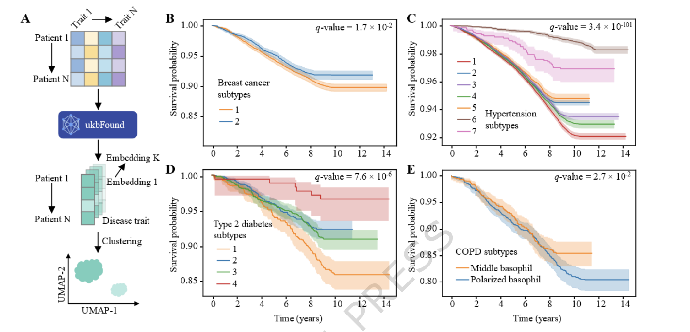
目标:找出同一种疾病下,具有不同预后(生存率)的亚组患者。
-
输入 (Input):
- 对象:特定疾病队列的所有患者(例如所有确诊 COPD 的人)。
-
数据表示:患者的
<CLS>向量。- 原文:“Specific disease cohorts were extracted and tokenized, which were processed into transformed patient embeddings… The special
<CLS>token… used as the aggregate individual representation.” - 即:把每个患者的完整体检数据输入 ukbFound,提取最后一个 Transformer 层
<CLS>位置的那个 256 维向量。这个向量代表了该患者“整体的健康状态”。
- 原文:“Specific disease cohorts were extracted and tokenized, which were processed into transformed patient embeddings… The special
-
处理 (Process):
- KNN 图 + Leiden 聚类:基于这些
<CLS>向量的距离,将患者分成不同的簇(Cluster)。
- KNN 图 + Leiden 聚类:基于这些
-
输出 (Output):
- 每个患者被标记为属于“亚组 A“、“亚组 B”等。
-
效果验证 (Evaluation):
-
生存分析 (Survival Analysis):
- 画 Kaplan-Meier 曲线,看不同亚组的存活率是否有显著差异(Log-rank test, FDR < 0.05)。
- 原文证据:“53/289 (18.3%) showing FDR-significant prognostic differences.”(证明分层有效,确实分出了预后不同的人)。
-
生物学解释 (Interpretability):
- 检查分出来的亚组在临床指标上是否有意义。
- 例如 COPD 案例:发现一个亚组的嗜碱性粒细胞(Basophil) 计数呈双峰分布,且该亚组肺功能下降更快(Fig. 2F, 2G, 2H)。这证明了模型找到的亚组不是随机噪声,而是有生物学依据的。
-
任务 2:多病共存网络(Multimorbidity Network Analysis)
图 4 任务 2:多病共存网络(Multimorbidity Network Analysis)
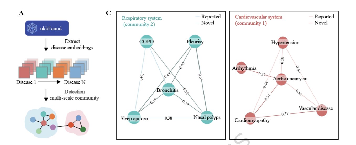
目标:发现疾病之间潜在的关联,画出“疾病知识图谱”。
-
输入 (Input):
- 对象:445 种疾病。
-
数据表示:疾病的“平均”向量 (Mean Disease Embedding)。
- 原文:“mean disease embeddings within each system were computed… The disease-level correlations were calculated by disease embedding’s cosine similarity.”
- 逻辑:既然 ukbFound 能生成患者的向量,那么把所有“患有高血压”的患者的向量取平均,就得到了“高血压”这个疾病在模型眼中的向量表示。
-
处理 (Process):
- 计算两两疾病向量之间的 余弦相似度 (Cosine Similarity)。
- 设定阈值(如 > 0.36),如果相似度高,就连一条线。
-
输出 (Output):
- 一个网络图,节点是疾病,连线强度代表关联度。
- 社区 (Communities):使用算法(Leiden)识别出一堆紧密连接的疾病群。
-
效果验证 (Evaluation):
-
文献重叠率 (Concordance):
- 将模型发现的连线与既往研究(遗传学、电子病历、疾病轨迹)对比。
- 原文证据:“Our results demonstrate substantial concordance with prior studies: 52.0% overlapped with genetically informed pairs…”(证明模型发现的关联是靠谱的)。
-
新发现 (Novelty):
- 找出文献中没报道过的连线。
- 例如:“low platelet disorder and gout”(血小板减少与痛风)。
-
任务 3:疾病预测(Disease Prediction)
图 5 任务 3:疾病预测(Disease Prediction)
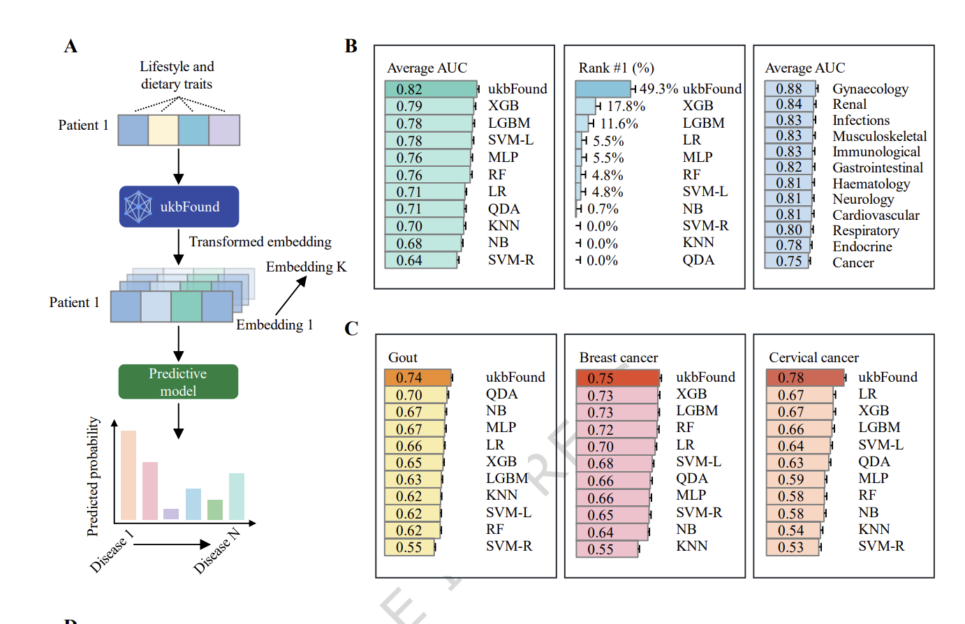
目标:仅凭生活习惯,预测未来患病风险(这是最考验模型泛化能力的)。
-
输入 (Input):
-
数据:仅包含生活方式和饮食特征的序列(排除所有疾病史和生化指标)。
- 原文:“using exclusively lifestyle and dietary habit traits… 465 lifestyle and dietary habit traits.”
-
数据表示:Token 级别的 Embedding 矩阵 (2D Matrix)。
- 注意:这里不使用
<CLS>向量,而是使用 Transformer 输出的整个序列。 - 原文:“pre-trained ukbFound model generates a 2D feature matrix where rows represent trait embedding vectors.”
- 形状:[序列长度, 256维度]。
- 注意:这里不使用
-
-
处理 (Process):
-
外接分类器 (Customized Classifier):
- 在 ukbFound 之上接了一个 TextCNN(文本卷积网络)。
- 原文:“Three parallel convolutional branches with kernel sizes corresponding to 2-, 3-, and 4-gram patterns then extract position-invariant local features… concatenated and processed through… classification layer produces disease predictions through individual sigmoid output units.”
- 这意味着:利用 CNN 捕捉生活习惯之间的局部组合模式(例如:吸烟+喝酒 组合在一起的风险 > 单独风险之和)。
-
-
输出 (Output):
- 一个概率值 (Sigmoid output),表示该个体患某种疾病(如痛风、乳腺癌)的风险。
-
效果验证 (Evaluation):
-
性能指标 (AUC):
- 对比 10 个基准模型(XGBoost, LightGBM 等)。
- 原文证据:“outperforming ten benchmark models by ΔAUC gains of +0.03 to +0.16.”(AUC 达到 0.82,远超传统机器学习)。
-
前瞻性验证 (Prospective Validation):
- 用基线健康的人做测试,看模型预测的高风险人群,是否真的在 8 年后发病了。
- 原文证据:“the highest-risk group showed 17.5-fold greater odds of developing gout up to 8 years in advance.”(高风险组的发病率是低风险组的 17.5 倍)。
-
可解释性 (SHAP):
- 分析是哪个特征导致了预测结果。
- 例如:预测痛风,模型显示“啤酒摄入”权重很高,符合医学常识。
-
代码是如何落实架构的
“ 通过审查作者提供的 ukbFound 核心预处理代码,我们不仅验证了上述架构的落地,还发现了一些论文中未详细披露的工程细节。 检查仓库发现里面的实现代码非常简洁,脚本不多,关键截取了里面的tokenizaiton的脚本以及train,model,loss的脚步来看,里面的逻辑和论文的一些关键设计契合。这篇文章应该是刚刚开源的。 ”
1. 确定性词表构建 (ValueVocab)
# 代码片段:确定性排序
sorted_by_freq_tuples.sort(key=lambda x: x[1], reverse=True) # 频次降序
# 结合先前的字母序排序,保证每次运行生成的 Token ID 完全一致解读:医疗模型的可复现性至关重要。作者通过稳定的排序策略,确保了 Value 词表的确定性,避免了训练时的随机漂移。
2. 双通道数据序列化 (tokenize_batch)
# 代码片段:返回分离的 Traits 和 Values
tokenized_data.append((traits, values, mod_types))解读:这里 traits 和 values 是作为两个独立的数组返回的。这直接对应了架构中的 “Dual-Vocabulary” 设计。模型在 Forward 阶段会分别进行 Embedding 查找后相加。
3. 预训练掩码策略:分层与强制 (random_mask_value) 🌟
def random_mask_value(values, mask_ratio=0.15, ...):
    # 1. 基础随机掩码 (Stratified Masking)
    n_mask = int(len(non_padding_idx) * mask_ratio)
    mask_idx = np.random.choice(non_padding_idx, n_mask, replace=False)
    row[mask_idx] = mask_value # mask_value 通常对应 -1 或 [MASK] ID

    # 2. 强制疾病掩码 (Forced Masking)
    # hqy 20240820 for 20002, force include diseases
row[(1302 <= row) & (row <= 2353) & (row % 2 == 0)] = mask_value细节发现:(没有在论文中提到的)
- 执行顺序与配额:代码显示,先执行 15% 随机掩码,再执行疾病强制掩码。这意味着疾病掩码是额外叠加的 (Union),不扣除 15% 的预算。这确保了稀疏的疾病信号(Disease Sparsity)能被模型充分学习。
- Magic Numbers (
1302-2353):这极有可能是作者内部处理后的疾病类 Trait 索引范围。20002是 UK Biobank 中 “Self-reported non-cancer illness” 的 Field ID。 - Mask 发生在哪个阶段?:注意
row[mask_idx] = mask_value操作的是整数数组 (ID)。这意味着 Mask 发生在 Embedding 查找之前。模型接收到的输入已经是带有[MASK]ID 的序列,进入 Embedding 层后才会转化为 Mask 向量并与 Trait 向量相加。
“ 但是笔者注意到这里有一个问题导致这里的源码不好直接使用: ”
- 问题:疾病索引范围
1302-2353硬编码在掩码函数中。 - 风险:如果更换数据集(如从 UKB 换成中国队列),疾病 ID 范围完全不同,代码将静默失效或错误掩码。
-
笔者建议:将疾病 ID 范围提取为配置文件(Config)或函数参数。
#比如说这样
def random_mask_value(..., force_mask_ranges=None):
    if force_mask_ranges:
        for start, end in force_mask_ranges:
            row[(start <= row) & (row <= end)] = mask_value
4. 损失函数 (masked_mse_loss 等)
笔者审查了来自loss.py脚本提供的 masked_mse_loss 和 criterion_neg_log_bernoulli 代码。Loss 不是用于预训练 MLM 的,而是用于下游微调任务(Downstream Tasks)的。
- 预训练 Loss:论文公式 (11) 明确指出使用的是
CrossEntropyLoss,用于在 47,066 维词表中预测被 Mask 掉的 Token。(就是传统Transformer框架的那种) - 下游 Loss:
BernoulliLoss 用于预测疾病发生的二分类任务,MSELoss 用于预测连续变量
遗留问题
论文提到 “mask budget (15%) was split equally between trait tokens and value tokens whenever both were present”,说明代码外层会有一个循环,分别对两个数组应用相同的 15% 随机策略(Trait 侧可能没有疾病强制掩码,或强制掩码逻辑不同)。
⚠️ 不确定性说明:我目前找到的代码仅展示了 random_mask_value,未展示 random_mask_trait 或外层调度逻辑。按理来说应该会在统一的一个代码层里面调用,不知道是不是我眼花没看到,有找到的读者可以告诉我。😵💫
针对该架构的一些细节问题
“ 笔者在阅读的时候提到了一些问题,分享出来也许可以解决你的疑惑,大家可以选择性阅读,当然读了之后肯定对架构理解会更透彻: ”
1. 关于 Yes/No 的编码:是否需要特定设计?
“ 回答:不需要针对特定 Trait 设计 Value Token,是全局通用的。 ”
“ 这个是我看论文的疑惑,后来在代码中得到解答 ”
- 代码:
在 random_mask_value 函数之前的代码中,并没有看到为特定疾病创建特殊的 Value ID。
论文原文提到:“For multi-select traits, each choice was converted into a binary single-select trait using ‘yes’ or ‘no’ tokens.”
- 解释:
模型只有两个通用的 Value Token 用于所有多选项(MST)特征:Token_Yes 和 Token_No。
区分“是什么病”不靠 Value Token,而是靠 Trait Token。
-
例如:
- Trait ID 100 (代表“高血压”) + Value ID (代表“Yes”)
- Trait ID 101 (代表“糖尿病”) + Value ID (代表“No”)
这种设计极大地压缩了 Value 词表的大小,使得模型只需要判断“有没有”,而具体的语义由 Trait 词表承载。
2. 关于初始化(Initialization):复杂 Embedding 怎么保证训练?
回答:基于源码和原文,没有特殊的初始化,而是依赖标准的 Embedding Lookup 和 Transformer 默认初始化。
- 原文提到:“We use the conventional embedding layers (PyTorch embedding layer)…”
以及 “The model was implemented in PyTorch v1.13.1…”
- 解释:
在 PyTorch 中,nn.Embedding 默认使用标准正态分布初始化权重。
这里没有特殊的预初始化技巧。 为什么能训练好?
- Warmup 机制:通常 Transformer 训练会有学习率 Warmup,防止一开始梯度爆炸。
- Masking 的强制学习:由于一开始所有 Embedding 都是随机的,模型预测肯定不准。但 Masking 任务(MLM)是一个强监督信号(Ground Truth 是确定的 ID),通过巨大的数据量(50 万人)和 50 个 Epoch 的迭代,梯度会迅速修正这些随机向量,使相关的 Trait 和 Value Embedding 在空间中靠近。
3. 关于疾病条目的判断:范围是否过小?
回答:范围确实受限于硬编码,但对于预训练任务是“够用”的。
- 代码:
在 random_mask_value 函数中有一行的硬编码:
# hqy 20240820 for 20002, force include diseases
row[(1302 <= row) & (row <= 2353) & (row % 2 == 0)] = mask_value- 范围小不小?
只覆盖了 20002 这一类疾病(以及可能的 ICD 编码)。但是,对于 MLM 任务来说,只要模型学会了“根据其他特征(如高血压、吸烟、年龄)推断出疾病(如冠心病)”,它就学到了疾病与表型的关联。
4. Masking 与 Embedding 融合的先后顺序
回答:先 Mask ID,后 Embedding 相加。二者是解耦的,但输入层面是融合的。
-
数据流:
- Tokenize 阶段(代码
tokenize_batch):生成trait_id数组和value_id数组。此时数据还是整数 ID。 -
Masking 阶段(代码
random_mask_value):直接修改整数数组。- 如果命中掩码,代码将数组中的数字(如
1350)改为-1(mask_value)。 - 此时还没有涉及 Embedding 查找!只是 ID 变了。
- 如果命中掩码,代码将数组中的数字(如
-
Embedding 阶段(模型 Forward 过程):
emb_t(trait_id)查找 Trait 向量。emb_v(value_id)查找 Value 向量。- 相加:
h = emb_t + emb_v。
- Tokenize 阶段(代码
-
为什么这样设计?
- 如果我们要预测“高血压(Yes/No)”,我们会把
Value IDMask 掉。 - 此时输入给 Embedding 层的
Value ID变成了[MASK]对应的 ID。 - 相加后的向量 hh =
Trait_Embedding("高血压")+Value_Embedding("[MASK]")。 - 妙处:模型知道这个位置是“高血压”特征(因为 Trait ID 没被 Mask,或者 Trait ID 也有对应的 Mask 策略),但它不知道值是 Yes 还是 No(因为 Value ID 被换成了 [MASK])。
- 所以,预测的时候,模型只需要看这个位置最终输出的向量,去分类器里预测 Value 是 Yes 还是 No。
- 如果我们要预测“高血压(Yes/No)”,我们会把
5. Masking 规则:是每个个体不一样吗?
回答:每个个体(每一行)都不一样,且每次看到都不一样(动态随机)。
- 代码:
在 random_mask_value 中:
for i in range(len(values)): # 遍历 batch 中的每一个样本
    row = values[i]
    non_padding_idx = np.nonzero(row - pad_value)[0] # 找出非 padding 的位置
    n_mask = int(len(non_padding_idx) * mask_ratio) # 计算要 mask 多少个
    if n_mask > 0:
        mask_idx = np.random.choice(non_padding_idx, n_mask, replace=False) # 随机抽取!
row[mask_idx] = mask_value解释:
np.random.choice是随机的。- 这意味着同一个病人,在 Epoch 1 被 Mask 掉的可能是“高血压”,在 Epoch 2 被 Mask 掉的可能是“糖尿病”。
- 这迫使模型必须全面掌握所有特征的关联,而不能只记住某几个特征的组合。
6.. CLS Token 的聚合原理
回答:通过 Self-Attention 的“注意力权重”自动学习聚合。
- 原文:
“A special CLS token is prepended to each sequence, and its final-layer embedding… is used as the aggregate individual representation.”
-
机制解析:
- 初始化:CLS 是一个可学习的向量,一开始它什么都不知道。
-
第一层 Attention:CLS 作为 Query,去询问序列里所有的 Token(身高、血压、疾病…)。
- 如果这个人的“身高”和“体重”都很高,Attention 机制可能会让 CLS 更多地关注这两个 Token 的 Value。
- CLS 收集了所有 Token 的信息,更新了自己的向量。
- 深层网络:经过 8 层这样的操作,CLS 向量就变成了一个高度浓缩的特征向量。
- 结果:这个向量代表了“这个人整体的健康状况”。下游任务(如预测死亡率)不需要看具体的血压是多少,只需要看这个 CLS 向量就够了。
架构设计:对 Transformer 的特定问题改造
“ ukbFound 的成功,本质上是通用架构 (Transformer) 与特定领域问题 (医疗表型) 深度适配的结果。针对特定的问题做出适配性的改进,是让我们的model的适用开发范围更加广泛的方法。 ”
-
从 Sequence 到 Set 的思维转变:
- 问题:医疗数据没有固定的先后顺序,且特征维度极高且稀疏。
- 方案:引入 Position-Free Embedding。模型通过 Self-Attention 的 QKTQKT 矩阵自动学习特征间的共现概率,而不是依赖位置编码。这与 Deep Sets 和 Set Transformers 的理念不谋而合。
-
从 ICD 到 Deep Phenotyping 的升级:
- 问题:传统的 Med-BERT/BEHRT 仅使用诊断编码(ICD),丢失了大量早期风险信号(如生活方式、生化指标)。
- 方案:Hierarchical Tokenization 将连续变量离散化(Q1-Q4),将多选变量二值化(Yes/No),使得所有异构数据都能映射到统一的 Token 空间中。
-
解决数据稀疏性的策略:
- 问题:疾病在健康人群中是极度稀疏的(正样本极少)。(这个在之前的Dephi论文处理human disease history也有padding token的处理。不过这里增加了mask的额外处理,本质上是和他的无序性适配的。)
- 方案:Forced Masking。代码中的
1302 <= row <= 2353强制 Mask 疾病相关的 Value,迫使模型必须依赖其他非疾病特征(如身高、饮食、血压)来推断疾病状态,从而隐式地学习“表型 -> 疾病”的映射关系。
小结
“ 这篇论文和对应的源码向我们展示了一种“Foundation Model + Downstream Discovery”的新范式(或者是一种新的领域交叉发论文的套路?): ”
- 数据即语言:将复杂的医疗数据转化为 Token 序列,利用 LLM 的 Scaling Law 红利,通过海量数据(50万人)训练出通用的医学特征表示。
- 无监督预训练,有监督发现:模型在预训练阶段不需要任何标签(无需知道谁得了病),仅通过“完形填空”(MLM)就能学到深层的医学关联。
- 可解释的预测:通过 SHAP 值分析,模型不仅能预测风险(如痛风),还能指出关键风险因素(如啤酒摄入),这与临床医生的诊断逻辑高度一致。然后基于这个已被验证的特性提出一个看起来数据上自圆其说的新发现,这是无法验证的,但是发现了就是发现了嘛,可以被信任才是最重要的。
这种设计思路不仅适用于 UK Biobank,未来完全可以迁移到 All of Us 或 China Kadoorie Biobank 等更多样化的队列中。ukbFound 证明了:当 AI 架构足够灵活地适应领域特性时,数据本身就是最好的医生。
笔者的话
“ 学习这篇论文花了我很多时间,这篇和之前的那篇Dephi可以做一个对比学习,同时也可以从这里看出学界对于这种交叉领域内容的偏好:虽然没有使用特别复杂的架构改进,但是可以做出一个相对来说自圆其说的结果来,使用的架构也不是最新的Transformer架构:比如这篇用的是LayerNorm,会增加模型训练负担,用的还是最原始那个配置,而且也没有测试SwiGLU类似的改进是不是可以使得Transformer可以学到更多内容,论文都是25年末发的顶刊,2篇nature,由此可见一斑,有时候探讨一个学科是否在时代风口上是一个好的倾向,甭管他是哪个风口。 其实依本人的拙见,所有架构的智能最后在理解语言,理解物理,理解事物之后,最重要的就是理解生命,这是现有的数据都无法预见的内化规律,又有哪个智能能在漫长的演化奇迹诞生的无数时间线中拥抱每一个生命的“灵魂”呢? ”